Truncation Sampling as Language Model Desmoothing

A language model (LM) specifies a distribution over sequences. But when using an LM, we rarely sample directly; instead, we modify the learned distribution via some algorithm, like nucleus sampling or top-k sampling. We call these methods truncation sampling algorithms.

These methods are hugely useful for generating high-entropy (high variety) text, and interestingly, more useful than, say, temperature scaling. But aren’t our language models quite good estimators? What is wrong with them such that the solution is truncation sampling? And have we figured out the right way to choose how to truncate?

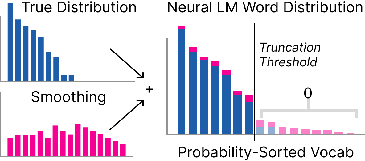
In this work, we argue that the problem is (uniform) smoothing; the LM hedging its bets by placing a little bit of probability mass everywhere. This might be due to early stopping and the KL divergence, and may remind you of classical n-gram language models.

In this view, the role of truncation sampling is to desmooth, attempting to recover the (support) of the true distribution and place 0 probability on any word that shouldn’t be allowed. In this view, we show that top-p unncessarily truncates many high probability words. Here’s a brief technical example of why; we’ll explain it later:

For example, for GPT-2 large and top-\(p\) with \(p=0.95\), top-\(p\) sampling truncates all words except Trump when generating for the prefix <|endoftext|> Donald. Why? Because (somewhat) high-probability words just outside the top 95% of the distribution are unnecessarily truncated.

We introduce eta-sampling, a simple truncation sampling algorithm that:

• Allows any word with probability above a fixed threshold, avoiding unnecessarily truncating (somewhat) high-probability words
• Allows any word with probability above a context-dependent threshold so that high-entropy distributions aren’t too heavily truncated
• Is less susceptible to repetition than top-\(p\) and typical decoding.
• Leads to more plausible long documents according to our raters in our study than top-$$p$4.
• Avoids previously unknown top-\(p\) problems in which low-entropy distributions are truncated very heaviliy, e.g., only allowing the word is after the prefix <|endoftext|> My name, when of course more options should be allowed.

This post is based on the following paper:

Truncation Sampling as Language Model Desmoothing
John Hewitt, Christopher D. Manning, and Percy Liang
Findings of EMNLP 2022 (long papers)

Truncation Sampling Algorithms

Intuitively, truncation sampling algorithms are those that:

• In autoregressive model sampling,
• for each individual conditional probability distribution as input,
• determine a subset of the vocabulary to “allow”,
• and reassign all probability mass from the complement of the allowed set to the allowed set.

In a bit of math, let \(\mathcal{V}\) be the vocabulary, let \(x\in \mathcal{V}\) be a word, and let \(P_\theta(x\mid x_{<i})\) be a conditional probability distribution (conditioned on a sequence of words \(x_{<i}\).) Let \(A\subseteq \mathcal{V}\); we call this the allowed set. A truncation sampling algorithm takes the conditional distribution as input and produces:

The key of any truncation sampling algorithm is how to choose the allowed set. Which words should be allowed at any timestep?

Perhaps the simplest common algorithm is top-\(k\) sampling, introduced by Fan et al., 2018. It allows the \(k\) most probable words. Holtzman et al., 2019 noted that sometimes the probability distribution amasses a most of its mass in fewer (or more) than the top \(k\) words; always allowing \(k\) words makes simple mistakes. Instead, they allow the minimal set of most likely words that keep \(p\) percent of the distribution’s mass: top-\(p\) (nucleus) sampling.

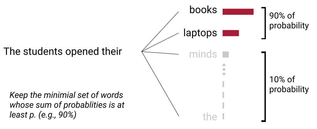
Other truncation sampling algorithms, with their own ways of determining the allowed set, often build off of these two; e.g., Typical Decoding (Meister et al., 2022) and mirostat (Basu et al., 2020).

Smoothing and Language Models

Consider for a moment an \(n\)-gram language model estimated via the maximum-likelihood estimate (counting.) Its probabilities are zero on almost the entire domain of \(\mathcal{V}^*\) because in any finite sample of data, most strings Here’s the probability distribution for a prefix \(x_{<i}\):

Is this a good estimate of the distribution over \(V^*\)? It depends on the metric by which you want to measure “good.” However, the KL-divergence is a useful notion of difference between distributions that is commonly used in the field, and by the KL-divergence this estimate is terrible. In particular, if any \(n\)-word sequence is observed at test time that wasn’t obsserved in the sample used for the MLE, the KL-divergence is infinite, since the probability assigned is \(0\).

Intuitively, not having observed a word at training time doesn’t mean the word can’t happen.

Smoothing is the process by the probability mass of a high-precision language model like an MLE \(n\)-gram model is spread out more, er, smoothly, across the domain of \(\mathcal{V}^*\). (Katz, 1987; Church and Gale, 1991) Useful \(n\)-gram smoothing can be quite complex, but a simple smoothing method is to just place a little bit of probability mass everywhwere, by interpolating the high-precision distribution with the uniform distribution.

Note now that all words (and through the chain rule, all sequences) now have non-zero probability, but the distribution is still mostly like the \(n\)-gram model. Intuitively, smoothing is important for scoring, since one wants to be able to rank the likelihood of noisy, low-quality text with different levels of noise. However, we argue that smoothing is bad for generation. Through smoothing, we now place probability mass on a wide set of strings that we would never want to generate, since they’re not high-quality language.

In the \(n\)-gram case with uniform smoothing, generating from smoothed vs unsmoothed models is pretty stark. Generating from an unsmoothed \(n\)-gram model, one is guaranteed local coherence (if the training distribution contains only coherent text) relative to the conditioning length \(n\), since every generated \(n\)-gram is guaranteed to have occurred in the training data. Generating from a uniform smoothed \(n\)-gram model, as soon as one generates outside the set of words with probability from the MLE estimate, the generation diverges wildly. Here’s an example:

Intuitively, once one samples off the support of the unsmoothed \(n\)-gram model, then the new prefix was never seen during the \(n\)-gram training, so its probabilities are undefined and one must fall back to the uniform distribution, generating nonsense.

One might ask whether smoothing is relevant for neural language models, since unlike \(n\)-gram models, we do not explictly smooth them after training. Neural language models use shared representations to provide estimates that naturally place probability mass on likely words in context that were not observed during training, part of the power they bring to bear on the estimation problem. We do not consider this smoothing for our purposes, but instead, generalization. Consider however two arguments for why neural LMs may be thought of as (uniformly) smoothed.

1. The KL-divergence loss when the LM observes a word during training approaches infinity quickly as the probability assigned to the word approaches zero. Unless absolutely confident a word could not appear in a given context, there is cause according to the loss to put a small amount of mass there.
2. Large language models are largely trained in a single epoch with early stopping, that is, each new minibatch of data they observe is brand new, meaning both that model training is stopped short of converging around the empirical training distribution and that the KL-divergence loss at each minibatch motivates the hedging we describe in point 1.

The goal of truncation sampling, then, is desmooth: to sample from the unknown unsmoothed distribution after observing only the smoothed distribution from the neural LM.

Principles of Desmoothing

In our paper, we describe a precise model for neural LMs in which they are implicitly smoothed by an unknown but uniform-like distribution, and show how two principles for performing desmoothing derive from that model. In this blog post, we’ll present the two principles, and defer to the paper for technical details. In both cases, the goal is to determine which words are likely to have probability mass only because of smoothing, and truncate those words while keeping all the words that likely have probability mass in the unsmoothed distribution.

The Absolute Probability Principle

The simple idea of the absolute probability principle in designing a truncation sampling algorithm is:

The absolute probability principle states: don’t truncate high-probability words.

From a desmoothing perspective, if one believes that only a small fraction of the probability mass of the neural LM is due to smoothing, and that mass is pretty spread out across a large vocabulary, then it’s unlikely that words with mass only due to smoothing have high probability.

While simple and intuitive, this is the principle that top-\(p\) decoding surprisingly breaks. Intuitively, in a vocabulary of say 50,000 and thus a uniform probability of \(1/50,000\), a probability of \(1-p\) (where \(p\) is 0.95, 0.99, etc.) is quite large; yet any word with at most that probability may be truncated. Here’s an example of just this in a GPT-2 model:

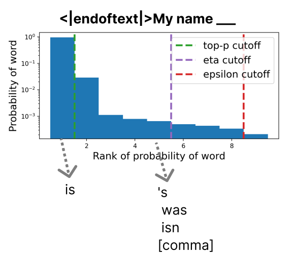
This plot shows the most likely words to continue the prefix <|endoftext|> My name, along with dotted lines showing the truncation cutoffs by top-\(p\) sampling (and some algorithms we’ve yet to introuce.) The most likely continuation is is; it achieves over 95% of the probability. Other good continuations, like 's, was, isn, and comma, are truncated by top-\(p\) sampling. Under our absolute probability principle, this means top-\(p\) sampling is losing out on some of the variety of language for no good reason; these probabilities are not likely due to smoothing, yet they’re truncated.

\(\epsilon\)-sampling

A simple algorithm that obeys the absolute probability principle is: just truncate any word with probability at most \(\epsilon\).

However, we do not recommend using \(\epsilon\)-sampling in practice, since it breaks our next principle:

The Relative Probability Principle

Intuitively, if one observes a high-entropy conditional distribution like the one produced by a language model for the prefix <|endoftext|> The, one wants to keep much of that variety. Here’s a plot of this conditional distribution; note how small the probabilities on the \(y\)-axis are.

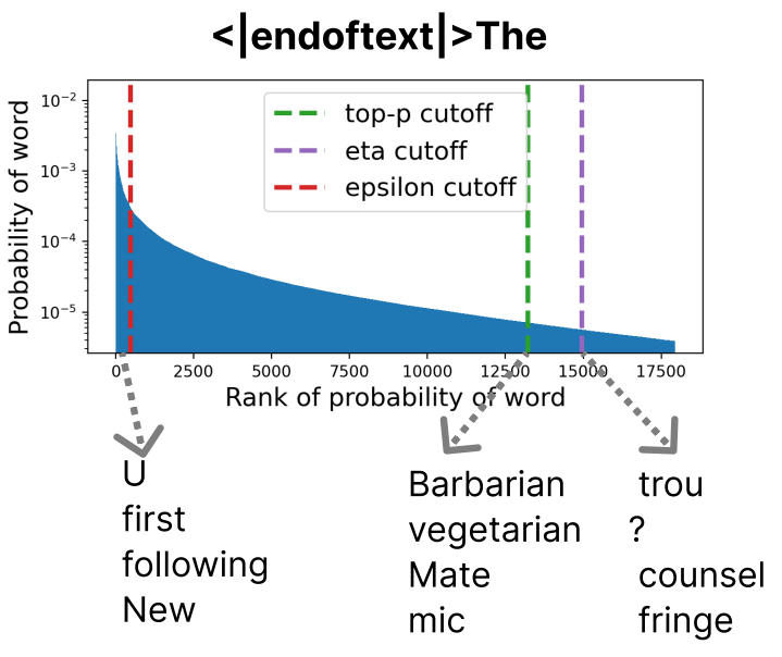
Intuitively, all words’ probabilities are small, so words whose probability comes only from smoothing should have probabilities that are small even relative to the other small probabilities.

Put another way, if a language model produces a high-entropy distribution, we hope that it does so because it has a lot of evidence for a lot of possible continuations, and so there’s less reason to smooth.

The relative probability principle states that in higher-entropy distributions, the probability threshold for truncating words should be closer to \(0\).

\(\epsilon\)-sampling does not obey the relative probability principle, and as shown in the plot above, truncates high-entropy distributions like <|endoftext|> The aggressively. Again, we think this is a key flaw of \(\epsilon\)-sampling, and do not think it should be used. High-entropy distributions often contain names, places, or things; it is not good to only be able to generate the most likely (in the training distribution) examples of the class.

Eta-sampling

Our proposed algorithm, \(\eta\)-sampling (“eta sampling”) respects both the absolute and relative probability principles. To do this, \(\eta\)-sampling allows words that meet either of two criteria. To respect the absolute probability principle, \(\eta\)-sampling allows any words above an absolute probability threshold, like \(\epsilon\)-sampling:

To respect the relative probability principle, \(\eta\)-sampling allows any words above an entropy-dependent probability threshold, defined as follows:

where \(\alpha\) is a scalar hyperparameter, and \(h_{\theta,x_{<i}}\) is the entropy of the language model’s conditional distribution for that prefix, \(h_{\theta,x_{<i}} = -\sum_{x\in\mathcal{V}} P_\theta(x\mid x_{<i}) \log P_\theta(x\mid x_{<i})\).

Why this threshold? Consider that \(\exp(-h_{\theta,x_{<i}})\) is the probability assigned to all elements in a uniform distribution with entropy \(h_{\theta,x_{<i}}\). For example, if the entropy is two (bits), then we have that \(2^{-2}=0.25\). Intuitively, if we were to observe a uniform distribution, we’d have no reason to truncate any one word over another; we should allow all words. This bar ensures that. The addition of the hyperparameter \(\alpha\) allows us to tune the threshold (e.g., allow all words in slightly non-uniform distributions.)

To make \(\eta\)-sampling simple and effective, we came to the heuristic of setting \(\alpha=\sqrt{\epsilon}\), and so provide the final truncation decision as follows. The allowed set \(\mathcal{A}_{x_{<i}}\) is:

The name of the algorithm comes from the capital \(\eta\), which is an \(H\), often used to denote entropy.

Here’s an implementation:

import torch

def eta_truncate(logits, hyperparam):
  """
  Arguments:
    logits: Torch tensor of size (bs, vocab_size)
    hyperparam: scalar. Try, e.g., 0.001
  Returns:
    Eta-truncation logits
  """
  hyperparam = torch.tensor(hyperparam).to(logits.device)
  # Compute entropy
  logits = torch.log_softmax(logits, dim=-1) # in case unnormalized logits are passed
  probs = logits.softmax(dim=-1)
  entropy = -torch.sum(logits*probs, dim=-1)

  # Calculate the threshold as min of absolute and relative thresholds
  threshold = torch.min(hyperparam, torch.sqrt(hyperparam)*torch.exp(-entropy))

  # Zero-out the probabilities in the non-allowed set
  indices_to_remove = probs < threshold.unsqueeze(1)
  return logits.masked_fill(indices_to_remove, -1e15)

print(eta_truncate(torch.tensor([[i for i in range(10)], [i*4 for i in range(10)], [1 for i in range(10)]]).float(), 0.5))

Experiments & Results

In our experiments, we study the truncation behavior and long sample variety and quality of \(\eta\)-sampling compared primarily to top-\(p\) sampling. The descriptions we give here are brief; refer to the paper for details.

Setting hyperparams with MAUVE

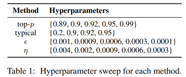
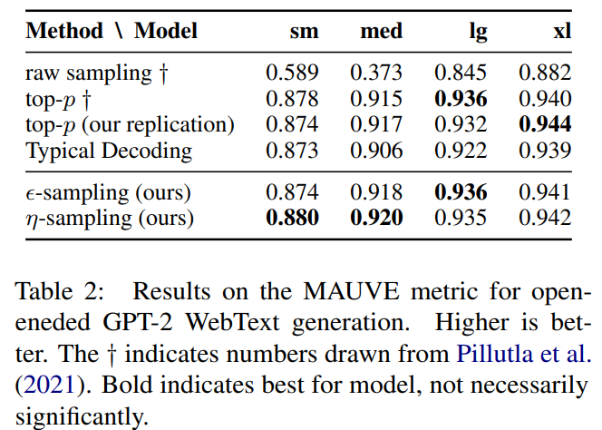
Truncation sampling methods tend to have a hyperparameter that controls the severity of truncation, so comparisons between methods need to determine how to set that hyperparameter. For most of our experiments, we set the hyperparameter to be that which maximizes the MAUVE score (Pillutla et al., 2021), an automatic metric of quality and diversity of generated text. The results are below, and all methods perform quite well relative to raw sampling, and not too differently from each other.

Long document plausibility, human judgments

Lest you think there’s no difference between the algorithms, however, also note that top-\(p\) and top-\(k\) aren’t well-distinguished by MAUVE; we use it just to set the hyperparameters. Now we get into our evlauations.

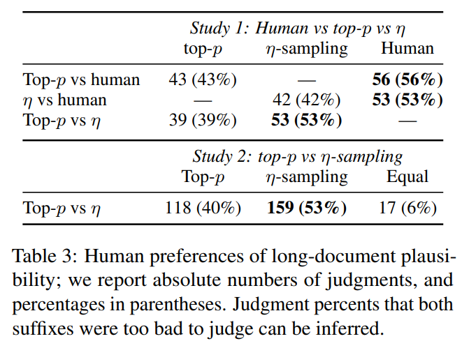
First, we generate long (900+ token) documents using top-\(p\) and \(\eta\)-sampling using shared prefixes (of 35 words) for which the real document was also at least 900 words. We show human annotators the shared prefix, and then a suffix of the document from pairs of the 3 options, and ask for a simple binary preference as to which suffix seems more plausibly could have come from the same document as the gold prefix (with an option to say they’re both too bad to tell.) This avoids asking annotators to keep the entire long document in working memory, a rather difficult ask.

We find that our annotators prefer the human document over both top-\(p\) and \(\eta\)-sampling from GPT-2 Large. Our annotators prefer our \(\eta\)-sampling over top-\(p\) as well. We ran a second study with new data and larger \(n\) to confirm the preference of our method, which we find is significant, and at a similar effect size.

Repetition Escape

We show in the paper (omitted here in the blog post) that top-\(p\) does in fact aggressively truncate low-entropy distributions on average compared to \(\eta\)-sampling. We hypothesize that this contributes to a tendency to degenerate into repetition (especially for high truncation rates), since repetition is guaranteed if the lower-probability non-repetition-continuing words are truncated.

To stress test this, we develop a toy setting in which we artificially introduce repetition into a naturalistic prompt, and measure the fraction of times that sampling methods fail to break the pattern of repetition.

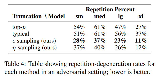
We do in fact find that our \(\eta$-sampling leads to lower rates of repetition (as does $4\epsilon\)-sampling; the reason \(\epsilon\)-sampling has even less repetition is that the MAUVE-maximizing hyperparameter led to a more lenient absolute probability threshold.)

CheckList-style Distribution Tests

Qualitatively, are the truncation sampling algorithms making the right truncation decisions? In these CheckList-style experiments (Ribeiro et al., 2020), we plot the truncation decisions of top-\(p\), \(\epsilon\)-sampling, and \(\eta\)-sampling for various prefixes.

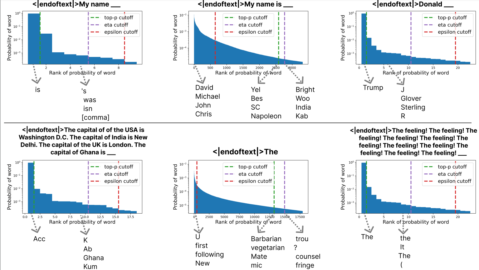
Take a look at the results below. The heavy truncation of top-\(p\) in low-entropy distributions is quite striking, allowing only a single possible continuation when intuitively many should be possible. Further, the heavy truncation of \(\epsilon\)-sampling in high-entropy distributions is undesirable. In each case, \(\eta\)-sampling makes a reasonable truncation decision.

We do note, however, that in a “prompting”-style prefix, top-\(p\) truncates all continuations but the beginning of the correct answer, which may be desirable.

Conclusion

The truncation we apply to our language models in order to avoid generating nonsense has a massive impact on the type of text that ends up generated, and it’s important to know what kinds of distributions and what kinds of words are being truncated.

We’ve attempted to characterize some of the understudied “local” effects of truncation, in terms of distribution entropy, but the sequence-level effects are going to be quite difficult to understand because of the increasing complexity of iteratively applying truncation to each new word.

Overall, however, truncation sampling algorithms are ubiquitous and useful. We hope that our work provides a useful way to think about the local aims of the methods, and our \(\eta\)-sampling provides a drop-in replacement for top-\(p\) that performs better and avoids some of the pitfalls we’ve mentioned.